Introduction to Statistics in Finance#

Many fields in finance rely on some sort of data analysis

For example fundamental analysis of a business:
- various numbers from the company itself (i.e. from the balance sheet)
- indicators representing the overall market

Results drive decisions, e.g. for an investement

There are many well established techniques and statistics for pricing financial products.

Some techniques more prominent since the dawn of powerful algorithms and artificial intelligence

Returns#

In order for an investment to be profitable, the money it yields must be higher than the inital investment made (plus transaction costs).

Assess so called return, usually discrete: relative change in investment value $S$.

\[ r_t = \frac{S_t - S_{t-1}}{S_{t-1}} =\frac{S_t}{S_{t-1}} - 1 \]

Note here that one time step $t$ is of arbitrary length, e.g. daily or monthly

Additivity#

Returns my be based on different time spans $\rightarrow$ aggreagte somehow

The property we are looking for is called addititvity: sum shorter-scale returns to get the larger-scale returns

Note that we can’t just split monthly returns into daily returns, this requires making assumptions on the distribution

Daily and weekly returns:
To calculate weekly returns from daily returns, we mustn’t use the daily return as is.

time $t$	0	1	2	3	4	5	6	7
prices $S_t$	100	110	121	110	132	105	112	105
return $r_t$	—	0.10	0.10	-0.09	0.2	-0.20	0.07	-0.06

If we simply added all returns, we’d find a weekly return of $r_{0,7} = 0.12$.
However, using the formula from above, we find that $$ r_{0,7} = \frac{S_7}{S_{0}} - 1 = \frac{105}{100} - 1 = 0.05 $$ and conclude that indeed daily returns cannot simply be added up in order to yield the weekly return.

We can calculate discrete returns simply by using a method of a Series object: .pct_change().
Note the NaN value for the first line.

df = pd.DataFrame({
    'S': [100, 110, 121, 110, 132, 105, 112, 105],
    },
index=list(range(8)))
df

	S
0	100
1	110
2	121
3	110
4	132
5	105
6	112
7	105

df['discrete_returns'] = df['S'].pct_change()
df

	S	discrete_returns
0	100	NaN
1	110	0.100000
2	121	0.100000
3	110	-0.090909
4	132	0.200000
5	105	-0.204545
6	112	0.066667
7	105	-0.062500

Portfolios and cross-sectional additivity#

A portfolio is a collection of investments, e.g. stocks. Portfolios are allocated differently, i.e., by a degree of risk. We can describe a portfolio’s value by the sum of the value of its constituents.

We define the value of a single position $i$ by multiplying the number of stocks $N_i$ with the stock value $S_i$

\[ P_i = N_i \cdot S_i \]

The Total portfolio value is the sum of all position values:

\[ P = \sum_i P_i = \sum_i N_i \cdot S_i\]

The weight of company $i$ in the portfolio is then

\[ w_i = \frac{P_i}{P} = \frac{N_i \cdot S_i}{\sum_j N_j \cdot S_j}, \sum_i w_i = 1\]

With those weights, we can calculate the portfolio return (cross-sectional additivity) as weighted sum of the company returns $R_i$:

\[ R_p = \sum_i w_i \, R_i \]

We talk about a naive portfolio of $J$ stocks when all weights are equal $w = w_1 = w_2 = ... = w_J$. In this case, the weighted sum becomes the mean of all stock returns $R_i$, as $w = \frac{1}{J}$ and the portfolio return is

\[R_p = \frac{1}{J} \sum_i^JR_i = mean(R_i)\]

Portfolio return and cross-sectional additivity#

We can show that property using the definitons from above

Price evolution for single stock $i$:

\[ P_{t+1}^i = P_t^i \,(1 + r_{t+1}^i) \]
Plugging this into the Portfolio value:

\[ P_{t+1}^{PF} = \sum_i P_{t+1}^i = \sum_i P_t^i \,(1 + r_{t+1}^i)\]

With the “regular” formula for discrete returns, the Portfolio return is:

\[ r_{t+1}^{PF} = \frac{P_{t+1}^{PF}}{P_t^{PF}} - 1 = \frac{\sum_i P_t^i (1 + r_{t+1}^i)}{\sum_j P_t^j} - 1 = \sum_i \frac{P_t^i}{\sum_j P_t^j}(1 + r_{t+1}^i) - 1 = \sum_i w_i\,(1 + r_{t+1}^i) - 1 = \sum_i w_i\,r_{t+1}^i \]

Let’s have a look at the following data:

time $t$	0	1	2	3	4	5	6	7
company A $A_t$	100	110	121	110	132	105	112	105
company B $B_t$	100	120	124	118	117	135	128	115

For simplicity, we will assume to invest the same amount of money in both stocks. This gives initial portfolio weights $w_1=w_2=0.5$. For such a naive portfolio, we can then just apply the mean, i.e. the portfolio return on day $t$ is just the mean of all returns $r_{i,t}$ for all companies $i$.

Calculate the daily returns of the portfolio using pandas:

df = pd.DataFrame({
    'A': [100, 110, 121, 110, 132, 105, 112, 105],
    'B': [100, 120, 124, 118, 117, 135, 128, 115],
    },
index=list(range(8)))
df

	A	B
0	100	100
1	110	120
2	121	124
3	110	118
4	132	117
5	105	135
6	112	128
7	105	115

When we want to calculate the returns for a naive portfolio, we simply calculate the mean over all returns. This give us the daily (naive) portfolio returns over time.

df_prices_and_returns = df.copy()
df_prices_and_returns['A_return'] = df_prices_and_returns.A.pct_change()
df_prices_and_returns['B_return'] = df_prices_and_returns.B.pct_change()
# mean applied to axis=1, means we calculate the row mean (axis=0 will calculate the column mean)
df_prices_and_returns.loc[1:,'naive_pf_return'] = df_prices_and_returns.loc[1:,['A_return', 'B_return']].mean(axis=1)
df_prices_and_returns

	A	B	A_return	B_return	naive_pf_return
0	100	100	NaN	NaN	NaN
1	110	120	0.100000	0.200000	0.150000
2	121	124	0.100000	0.033333	0.066667
3	110	118	-0.090909	-0.048387	-0.069648
4	132	117	0.200000	-0.008475	0.095763
5	105	135	-0.204545	0.153846	-0.025350
6	112	128	0.066667	-0.051852	0.007407
7	105	115	-0.062500	-0.101562	-0.082031

We can apply .pct_change() to the whole dataframe, to create a new one with the same column names.

df_just_returns = df.copy()
df_just_returns = df_just_returns.pct_change()
df_just_returns

	A	B
0	NaN	NaN
1	0.100000	0.200000
2	0.100000	0.033333
3	-0.090909	-0.048387
4	0.200000	-0.008475
5	-0.204545	0.153846
6	0.066667	-0.051852
7	-0.062500	-0.101562

Characteristics of returns#

Usually, returns exhibit the following:

expected returns are close to zero (the shorter the time span, the smaller the expected return)
weakly stationary (i.e. constant expected value and variance over time) but usually volatility clustering
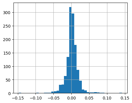
skewed distribution

From these items alone, we can start an analysis of stock returns by looking at some (standardized) moments of the empirical data:

the average return as an estimate of the expected return
the empirical variance or standard deviation/volatility

Use pandas, by calling the appropriate methods.

We will have a look at real-world data, downloading close prices using the yfinance package and calculating the returns.

import yfinance as yf

msft = yf.Ticker('MSFT')
msft = msft.history(
    start='2020-01-01',
    period=None
)

msft = msft[['Close']].copy()
msft['daily_disc_return'] = msft['Close'].pct_change()
msft.dropna(inplace=True)

avg_return = msft.daily_disc_return.mean()
vola = msft.daily_disc_return.std()

print(f'average return {np.round(avg_return,4)}')
print(f'volatility {np.round(vola, 4)}')

average return 0.0011
volatility 0.0191

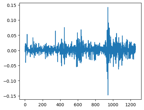
As we discussed in earlier chapter, it is always recommended to take a look at some charts.
We can plot returns over time as well as look at the distribution.

msft.daily_disc_return.plot()

<AxesSubplot:xlabel='Date'>

_images/13_financial_stats_CAPM_2025_24_1.png

msft.daily_disc_return.hist(bins=41)

<AxesSubplot:>

_images/13_financial_stats_CAPM_2025_25_1.png

	Date	daily_excess_return	daily_excess_return_sp
0	2020-01-03 00:00:00-05:00	-0.022452	-0.017060
1	2020-01-06 00:00:00-05:00	-0.007415	-0.006467

Data Visualisation and Reporting with Python

Introduction to Statistics in Finance

Contents