SciKit Learn#
The sklearn package provides a broad collection of data analysis and machine learning tools:
cover the whole process, data manipulation, fitting models, evaluating the results
Sklearn is based on numpy: data and results as numpy arrays.
Classes and functions are provided in an high-level API:
allows application without requiring (too much) knowledge about the algorithm itself
API allows to use the same syntax for very different algorithms
Basic syntax for creating a model:
instantiate the respective (algorithm’s) object with hyper parameters and options
fit the data using this object’s built-in methods
evaluate the model or use the model for prediction
Note: we import classes specifically from the scikit-learn package instead of importing the package as a whole
Regression#
Linear Regression#
in LR, we model the the influence of some independent numerical variables on the value of a dependent numerical variable (the target).
widely used in economics
The ordinary least squares (OLS) regression is found in module linear_model as the LinearRegression class.
NOTE: by default, sklearn will fit an intercept. To exclude the intercept, set fit_intercept=False when instantiating the LinearRegression() object.
To demonstrate the procedure, we will use a health insurance data set trying to explain the insurance charges.
The data includes some categorical variables, for which we need to create dummy variables
intercept y = \(\alpha\) + \(\beta\) \(\cdot\) x
no intercept y = \(\beta\) \(\cdot\) x
import pandas as pd
import numpy as np
df = pd.read_csv("data/insurance.csv")
#df = df.select_dtypes(include=['int64', 'float64'])
df.head(3)
| age | sex | bmi | children | smoker | region | charges | |
|---|---|---|---|---|---|---|---|
| 0 | 19 | female | 27.90 | 0 | yes | southwest | 16884.9240 |
| 1 | 18 | male | 33.77 | 1 | no | southeast | 1725.5523 |
| 2 | 28 | male | 33.00 | 3 | no | southeast | 4449.4620 |
transform the pandas Series for independent and dependent variable to a numpy array, which we reshape to 2D
instantiate the object (default option
fit_intercept=Trueincluded for illustrative reasons)call the
.fit()method with positional arguments: first the independent variable(s) X, then target y
After the fit, we can access the parameters: intercept and coefficient(s). Again, the syntax is similar as above for the StandardScaler.
In this example, we regress the charges for a policy on the age of the customer.
from sklearn.linear_model import LinearRegression

X = np.array(df.age).reshape(-1,1)
y = np.array(df.charges).reshape(-1,1)

linreg = LinearRegression(fit_intercept=True)
linreg.fit(X,y)

print(f"intercept: {linreg.intercept_}, coefficient: {linreg.coef_}")
intercept: [3165.88500606], coefficient: [[257.72261867]]
linreg.coef_
array([[257.72261867]])
What we find is a positive slope, linreg.coef_ > 0, meaning that a higher bmi results in higher charges. To be precise, if your bmi increases by one unit, you will, on average, be charged about 394 more units.
We can also see that the estimated parameters are returned as (nested) arrays. To get to the values, we must hence extract them accordingly.
print(f"intercept: {linreg.intercept_[0]}, coefficient: {linreg.coef_[0][0]}")
intercept: 3165.8850060630284, coefficient: 257.72261866689547
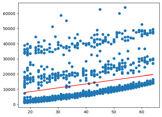
Now, we can generate fitted values and plot these together with the data to get a visualisation of the regression results
To do so, we pass the X values to the .predict() method and save the result as y_pred.
We then use matplotlib to create a scatter plot of the data and add a line plot of the regression line.
import matplotlib.pyplot as plt
y_pred = linreg.predict(X)

plt.scatter(X, y)
plt.plot(X,y_pred, color='red')
plt.show()
Better: statsmodels#
At this point, we shortly discuss an important point when it comes to regression: significance.
We skipped this above, because sklearn has its shortcomings when it comes to this kind of ‘classical statistics’. The calculation of p-values for example is not included and would have to be implemented by oneself.
For such statistics, we can switch to the statsmodels package:
maybe a better choice for regression modelling because of detailed output
Below, an example is given for the regression from above. The syntax is just slightly different:
we call
add_constanton the data (!) to fit an interceptwe instantiate an
OLSobject, providign the data here, not in the subsequentfitcallusing
.summary()automatically outputs a table of information about the model
intercept y = \(\alpha\) + \(\beta\) \(\cdot\) x
no intercept y = \(\beta\) \(\cdot\) x
import statsmodels.api as sm

X = sm.add_constant(df.age)
y = df.charges

res = sm.OLS(y, X).fit()

print(res.summary())
                            OLS Regression Results
==============================================================================
Dep. Variable:                charges   R-squared:                       0.089
Model:                            OLS   Adj. R-squared:                  0.089
Method:                 Least Squares   F-statistic:                     131.2
Date:                Wed, 04 Feb 2026   Prob (F-statistic):           4.89e-29
Time:                        12:04:18   Log-Likelihood:                -14415.
No. Observations:                1338   AIC:                         2.883e+04
Df Residuals:                    1336   BIC:                         2.884e+04
Df Model:                           1
Covariance Type:            nonrobust
==============================================================================
                 coef    std err          t      P>|t|      [0.025      0.975]
------------------------------------------------------------------------------
const       3165.8850    937.149      3.378      0.001    1327.440    5004.330
age          257.7226     22.502     11.453      0.000     213.579     301.866
==============================================================================
Omnibus:                      399.600   Durbin-Watson:                   2.033
Prob(Omnibus):                  0.000   Jarque-Bera (JB):              864.239
Skew:                           1.733   Prob(JB):                    2.15e-188
Kurtosis:                       4.869   Cond. No.                         124.
==============================================================================

Notes:
[1] Standard Errors assume that the covariance matrix of the errors is correctly specified.
\(H_0\) : \(\beta =0\)
We can access the quantities from the table specifically, using the names listed when running dir(res_smoker).
res.pvalues
const    7.506030e-04
age      4.886693e-29
dtype: float64
res.params
const    3165.885006
age       257.722619
dtype: float64
linreg.coef_
array([[257.72261867]])
linreg.intercept_
array([3165.88500606])
print(X.shape)
X.head(2)
(1338, 2)
| const | age | |
|---|---|---|
| 0 | 1.0 | 19 |
| 1 | 1.0 | 18 |
y.shape
(1338,)
y_pred_sm = res.predict(X)

plt.scatter(df.age, y)
plt.plot(df.age,y_pred_sm, color='red')
plt.show()